H and H2

import profess
import ase_tools
import matplotlib.pyplot as plt
import numpy as np

$H$ atom

The hydrogen atom potential is $v(\mathbf{r})=-\tfrac{1}{r}$ in atomic units. Solving the associated Schrödinger equation yields the ground state energy $E_0=-\tfrac{1}{2}$.

For a single, isolated electron, we may infer its wave function from the electron density, $\psi(\mathbf{r}) = \sqrt{n(\mathbf{r})}$. Furthermore, its kinetic energy is given exactly by the Weizsäcker functional,

$$ T_W[n] = \int \mathrm{d}\mathbf{r} , \sqrt{n(\mathbf{r})} \left(-\frac{1}{2}\nabla^2\right) \sqrt{n(\mathbf{r})}. $$

For this reason, we can obtain $E_0$ as a simple example of orbital-free density functional theory,

$$ E_0 = \mathrm{min}{n} \left[ T{W}[n] + \int \mathrm{d}\mathbf{r} , v(\mathbf{r}) n(\mathbf{r}) \right] \quad\text{with}\quad \int \mathrm{d}\mathbf{r} , n(\mathbf{r}) = 1. $$

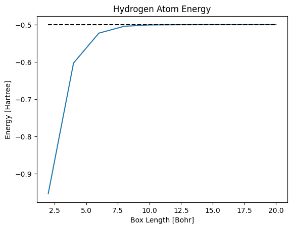
The following code implements this approach, showing that the energy indeed approaches $-\frac{1}{2}$ when the simulation box is sufficiently large.

planewave_cutoff_energy = 50
box_lengths = np.linspace(2,20,10)

energies = []
for box_length in box_lengths:
    system = (
        profess.System.create(box_length*np.identity(3), planewave_cutoff_energy)
        .add_coulomb_ions(1.0, [[0,0,0]], cutoff=0.5*box_length)
        .add_electrons()
        .add_weizsaecker_functional()
        .add_ion_electron_functional()
    )
    system.minimize_energy()
    energies.append(system.energy('h'))

plt.plot(box_lengths, energies)
plt.plot(box_lengths, -0.5*np.ones(box_lengths.size), 'k--')
plt.title('Hydrogen Atom Energy')
plt.xlabel('Box Length [Bohr]')
plt.ylabel('Energy [Hartree]')
plt.show()

One technical point: rather than the full Coulomb potential, the code uses a truncated version set to zero beyond a cutoff radius. This modification facilitates study of the isolated atom with periodic boundary conditions.

$H_2$ molecule

The electrons in an $H_2$ molecule share a single spatial orbital, so the Weizsäcker functional again provides the exact noninteracting kinetic energy. However, we must now incorporate electron-electron and ion-ion interactions, and the total system energy is

$$ E_0 = \mathrm{min}{n} \left[ T{W}[n] + E_H[n] + E_{xc}[n] + \int \mathrm{d}\mathbf{r} , v(\mathbf{r}) n(\mathbf{r}) + E_{II} \right] \quad\text{with}\quad \int \mathrm{d}\mathbf{r} , n(\mathbf{r}) = 2. $$

The following code explores the relationship between energy and bond length using the Perdew-Burke-Ernzerhof approximation for the exchange-correlation functional.

system = (
    profess.System.create(20*np.identity(3), 20)
    .add_coulomb_ions(1.0, [[0,0,0],[1,1,1]])
    .add_electrons()
    .add_weizsaecker_functional()
    .add_hartree_functional()
    .add_perdew_burke_ernzerhof_functional()
    .add_ion_electron_functional()
    .add_ion_ion_interaction()
)
    
distances = np.linspace(1,2,10)
energies = []
for d in distances:
    system.move_ions([[10-d/2,10,10],
                      [10+d/2,10,10]])
    energies.append(system.minimize_energy().energy())

fig, ax = plt.subplots()
ax.plot(distances, energies)
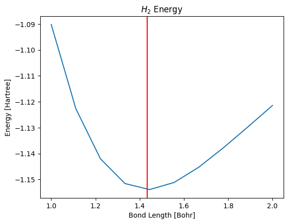
ax.set_title('$H_2$ Energy')
ax.set_xlabel('Bond Length [Bohr]')
ax.set_ylabel('Energy [Hartree]');

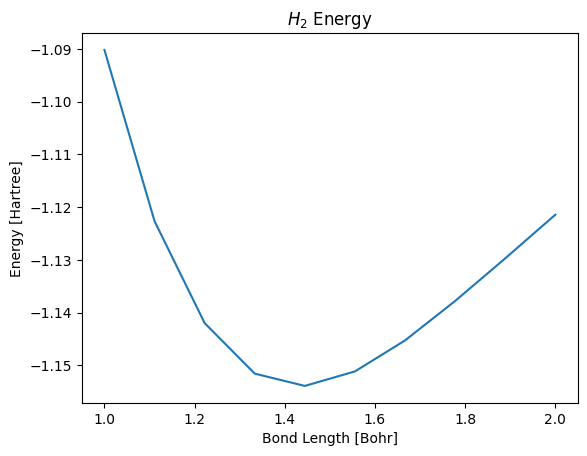
From the plot, it appears the equilibrium bond length is approximately 1.4-1.5 Bohr. To find a precise value, we allow the atoms to relax until all forces are minimized.

ase_tools.minimize_forces(system, 'BFGSLineSearch')

xyz_coords = np.array(system.ions_xyz_coords())
distance = np.sqrt(np.sum((xyz_coords[0,:]-xyz_coords[1,:])**2))
print('\nBond length after minimizing forces: {:4.2f} Bohr\n'.format(distance))

ax.axvline(distance, color='red')
fig

                Step[ FC]     Time          Energy          fmax
BFGSLineSearch:    0[  0] 09:54:14       -1.121424        0.0754

BFGSLineSearch:    1[  5] 09:54:29       -1.152840        0.0279

BFGSLineSearch:    2[  7] 09:54:36       -1.153926        0.0030

BFGSLineSearch:    3[  8] 09:54:38       -1.153936        0.0005

BFGSLineSearch:    4[  9] 09:54:39       -1.153937        0.0001

Bond length after minimizing forces: 1.43 Bohr