Aluminum

For face-centered cubic (FCC) aluminum, the build stage might appear as follows.

# choose box vectors and a planewave energy cutoff
box_vectors = 4.05 * np.identity(3)
energy_cutoff = 1200

# create the system
system = profess.System.create(box_vectors, energy_cutoff, ['a','ev'])

# add ions and electrons
system.add_ions(
    'potentials/al.gga.recpot',
    box_vectors[0,0] * np.array([(0.0,0.0,0.0),
                                 (0.5,0.5,0.0),
                                 (0.5,0.0,0.5),
                                 (0.0,0.5,0.5)]),
    'a')
system.add_electrons(system.total_ion_charge())

# add energy terms
(
system
    .add_wang_teter_functional()
    .add_hartree_functional()
    .add_perdew_burke_ernzerhof_functional()
    .add_ion_electron_functional()
    .add_ion_ion_interaction()
)

The usual next step is to modify the system with minimize_energy(), finding the ground state electron density and energy.

system.minimize_energy()

One can then print system properties, inspect the electron density, and more.

print('Volume (A3):        {:5.2f}' .format(system.volume('a3')))
print('Grid shape:         {:}'     .format(system.grid_shape))
print('Total energy (eV):  {:5.3f}' .format(system.energy('ev')))

Volume (A3):        66.43
Grid shape:         [25, 25, 25]
Total energy (eV):  -228.733

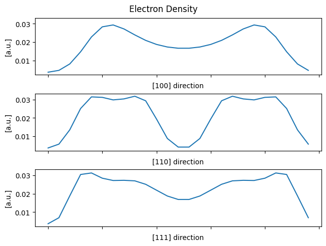
fig, ax = plt.subplots(3, 1, constrained_layout=True, sharey=True)
fig.suptitle('Electron Density')
ax[0].plot([system.electron_density[i,0,0] for i in range(system.grid_shape[0])])
ax[1].plot([system.electron_density[i,i,0] for i in range(system.grid_shape[0])])
ax[2].plot([system.electron_density[i,i,i] for i in range(system.grid_shape[0])])
for i, label in enumerate(('[100]', '[110]', '[111]')):
    ax[i].set_xlabel(label + ' direction')
    ax[i].xaxis.set_ticklabels([])
    ax[i].set_ylabel('[a.u.]')
plt.show()